The Simple Pendulum
When is the small-angle approximation good enough, and how does the integrator affect energy conservation?
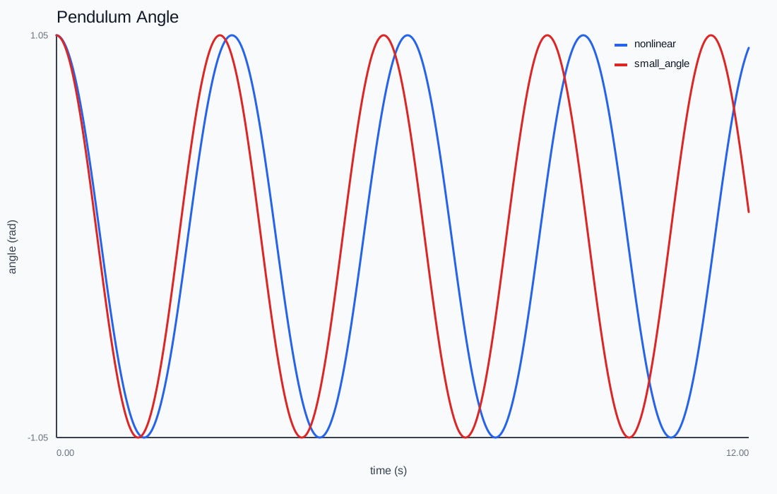
Drag the bob to set the starting angle, or change the length and gravity. The faint ghost is the small-angle approximation released from the same point — watch it drift apart at large amplitude.
Two equations, one pendulum
The real pendulum obeys \ddot\theta = -\tfrac{g}{L}\sin\theta; the textbook one replaces \sin\theta with \theta. The approximation is only good while the amplitude is small enough that those two agree — and the lab is built to show you exactly where it breaks.
Where it breaks
Start at 0.1, 0.5, and 1.0 rad. At 0.1 rad the nonlinear and linear curves are indistinguishable. By 1.0 rad the true period is noticeably longer — the restoring torque saturates because \sin\theta \lt \theta, so a wide swing takes its time. The small-angle model never knows this; it ticks at a fixed frequency forever.
The energy check
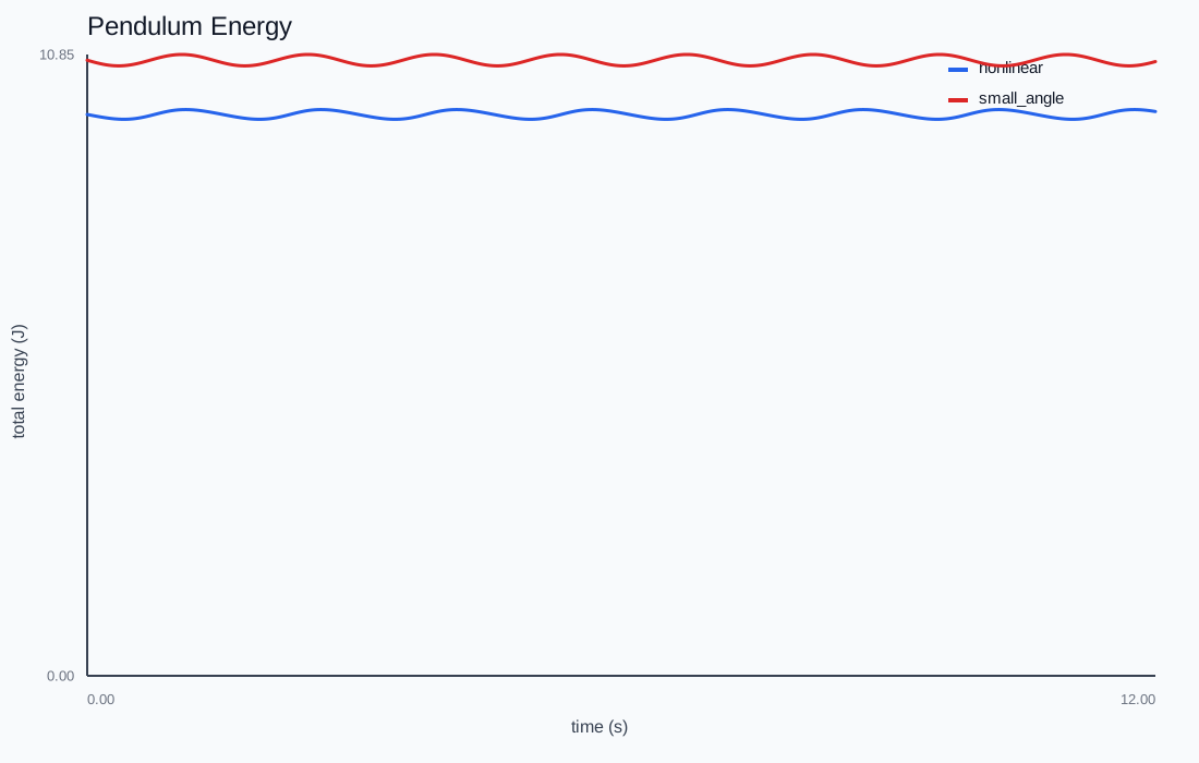
Because the swing is conservative, total energy should be flat. Watching it under different integrators and timesteps is the same lesson as the projectile lab: a non-symplectic step slowly pumps or bleeds energy, and the pendulum's amplitude wanders as a result.
This chapter is drawn from the physics-lab study notes and renders. The longer write-ups and project essays live on the blog.