The Ising Model

Can a phase transition emerge from a trivially simple rule, and how do you simulate a system at temperature T when you can't enumerate its 2^N states?

Interactive · live simulation

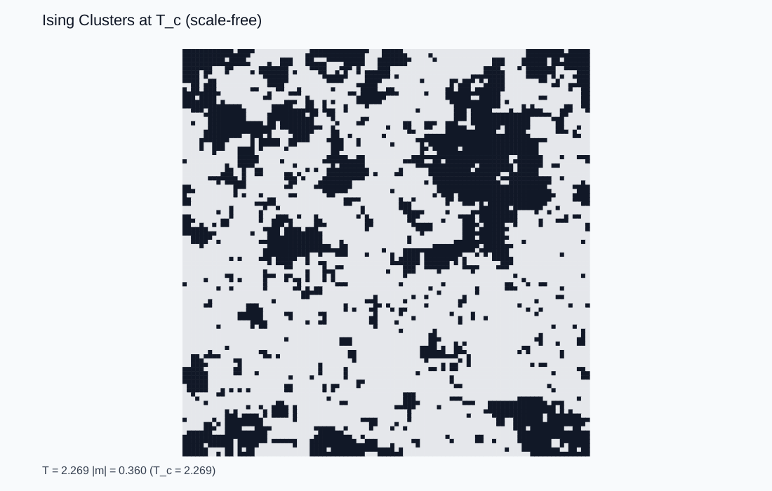
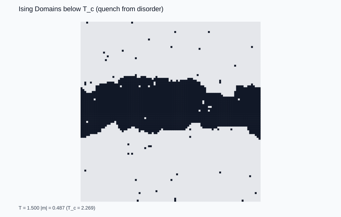
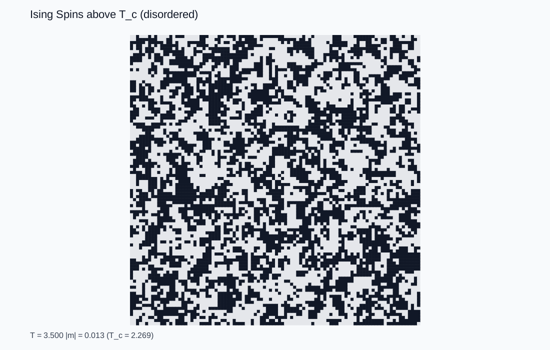
Drag the temperature through the critical point T_c ≈ 2.269 J and watch the lattice live. Cold: large ordered domains. Hot: salt-and-pepper noise. At T_c: clusters of every size at once.

The Ising Model — simulation render — fig 1. At the critical temperature: scale-free, fractal-looking clusters of every size at once — the hallmark of a diverging correlation length.

Neighbors prefer to agree

A square lattice of spins s = \pm 1 with energy E = -J\sum s_i s_j. Aligned neighbors lower the energy. That is the entire microscopic rule — and yet it produces a sharp, qualitative change in collective behavior at a critical temperature, exactly like a magnet losing its magnetism.

fig 2. Below T_c: large ferromagnetic domains, neighbors agreeing ~97% of the time.

Never compute Z

The partition function has 2^N terms, so direct evaluation is hopeless. The Metropolis algorithm samples the Boltzmann distribution anyway, using only energy differences: flip a spin if it lowers the energy, otherwise accept with probability \exp(-\Delta E/T). After enough sweeps the configurations are drawn from the correct thermal ensemble — the central trick of computational statistical mechanics.

fig 3. Above T_c: salt-and-pepper noise as entropy wins and spins flip freely.

The transition and its fingerprints

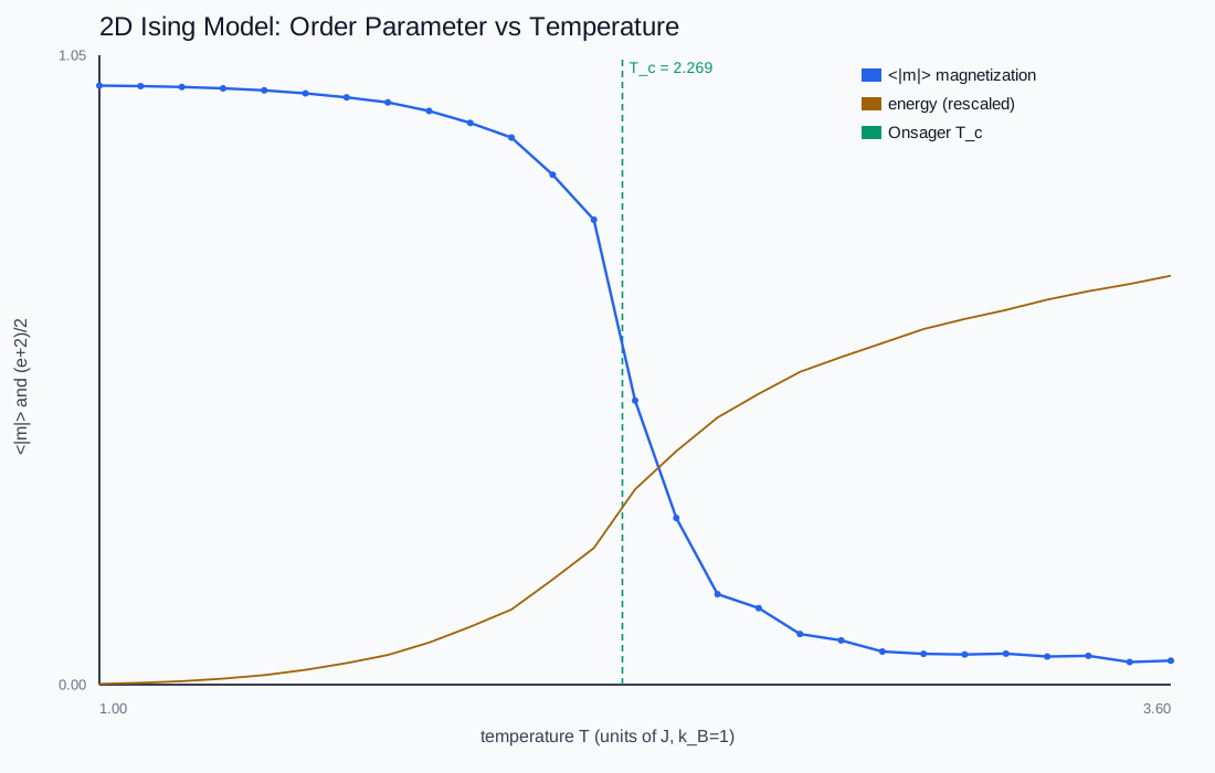
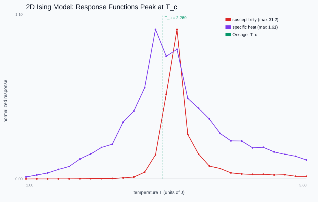
Sweep temperature and the magnetization holds near 1, then collapses through T_c = 2J/\ln(1+\sqrt2) \approx 2.269 — Onsager's exact result, reproduced on a 48×48 grid. The sharper fingerprints are the fluctuations: susceptibility and specific heat both peak at T_c, because the system poised between order and disorder responds enormously to tiny perturbations.

fig 4. The order parameter ⟨|m|⟩ holding near 1, then collapsing sharply through T_c ≈ 2.269 J — Onsager's exact value, reproduced.

fig 5. Susceptibility and specific heat both peaking at the transition: near T_c, tiny perturbations produce huge responses.

This chapter is drawn from the physics-lab study notes and renders. The longer write-ups and project essays live on the blog.