Quantum Eigenstates

How do you find the energy eigenstates that set spectral lines and bonding — without diagonalizing a giant matrix?

Interactive · live simulation

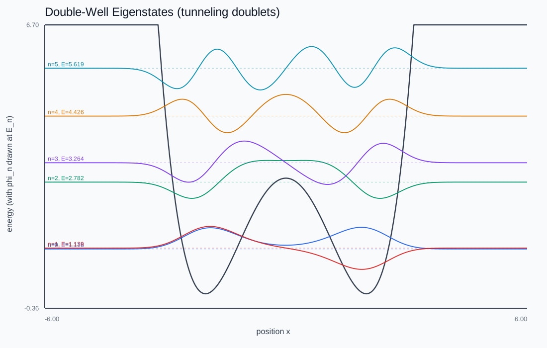
Imaginary-time relaxation finding the eigenstates live: a random guess decays onto the ground state. Hit "Next state" to project it out and climb the ladder. Try the double well and watch the tunneling doublet appear.

Quantum Eigenstates — simulation render — fig 1. A double well: the low states form tunneling doublets — a symmetric state just below an antisymmetric one — the toy model behind the ammonia inversion line and bonding/antibonding orbitals.

Rotate time into the imaginary axis

Substitute t = -i\tau into the Schrödinger equation and it becomes a diffusion equation \partial\psi/\partial\tau = -H\psi. Every energy component decays as \exp(-E_n\tau), but the lowest decays slowest. Renormalize after each step and any starting state relaxes onto the ground state — no matrix diagonalization, just the same tridiagonal Hamiltonian from the previous lab.

fig 2. The harmonic oscillator: the evenly spaced ladder E_n = n + ½, reproduced to better than 1e-3.

Climbing the ladder

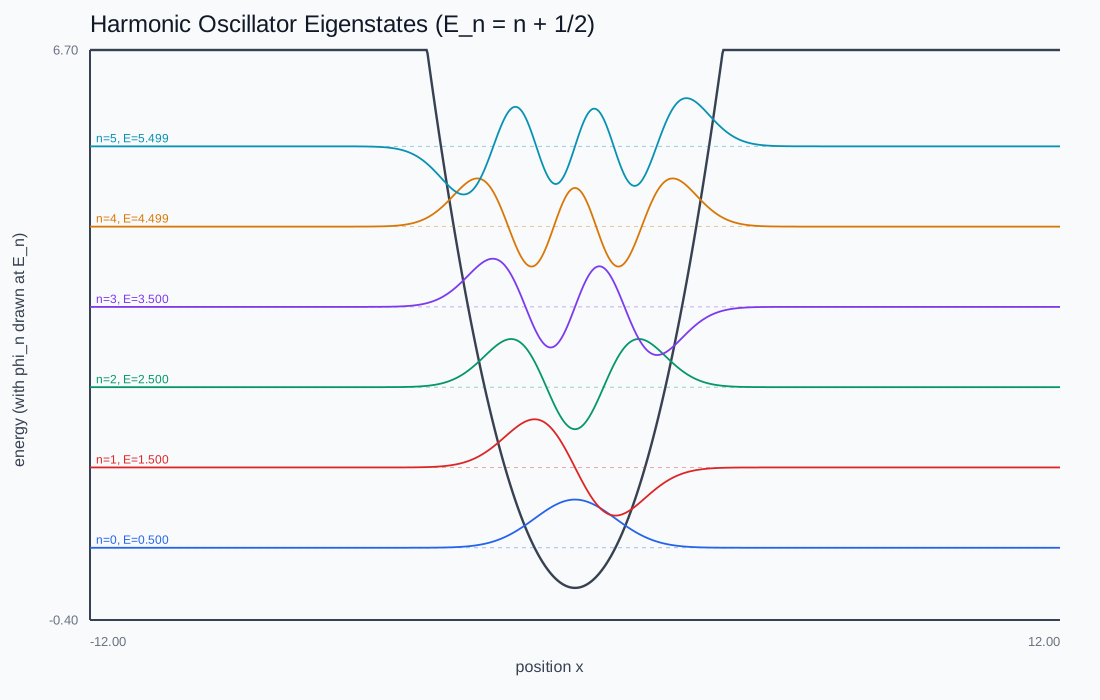
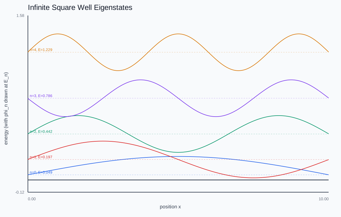
To get excited states, relax again while projecting out every already-converged lower state (Gram-Schmidt). The slowest-surviving component is then the next eigenstate. The states come out orthonormal by construction, checked to 1e-6.

fig 3. The infinite square well: energies following (n+1)²π²/2L², with higher states acquiring a small lattice-dispersion bias.

Backward Euler, not Crank-Nicolson

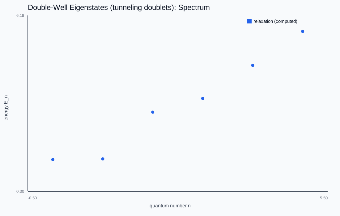
CN's amplification factor tends to -1 for high-energy lattice modes, so the relaxation gets stuck on the spurious zigzag mode. Backward Euler's factor 1/(1+\Delta\tau\,E) decreases monotonically with energy — high modes damped hardest — and the energy is read off as an exact Rayleigh quotient regardless of step accuracy. The double well's tunneling doublets are the payoff: the toy model behind molecular inversion lines and bonding pairs.

fig 4. The double-well spectrum, showing how doublet splittings grow with energy as the barrier becomes more penetrable.

This chapter is drawn from the physics-lab study notes and renders. The longer write-ups and project essays live on the blog.