Maxwell FDTD

A changing E makes a changing H and vice versa; the two leapfrog through space as light. How do you simulate fields that generate themselves?

Interactive · live simulation

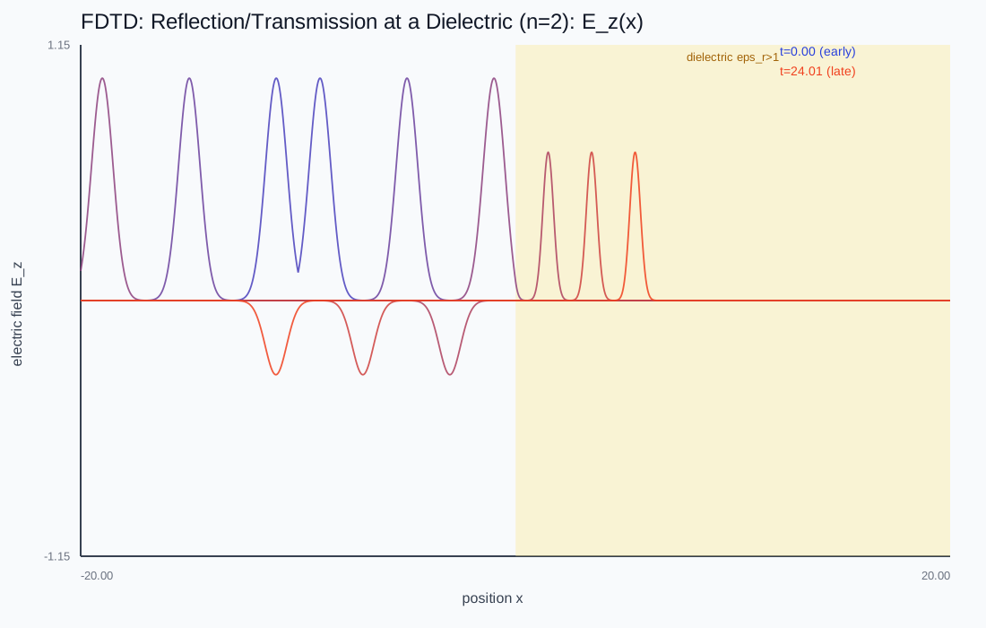
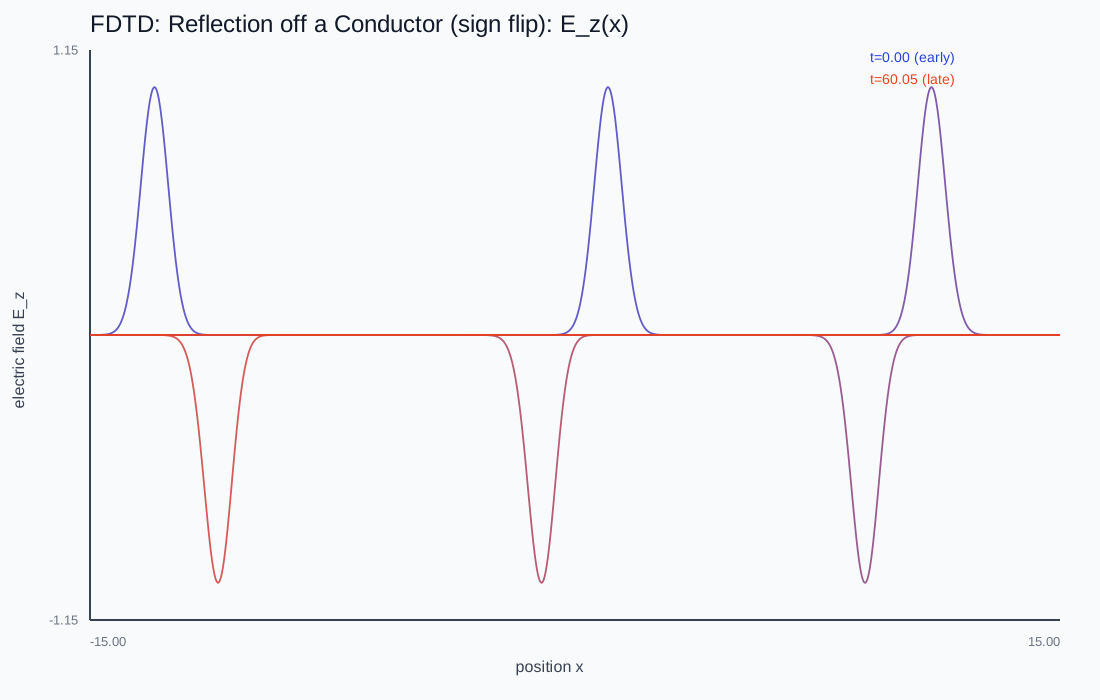
A 1D Maxwell FDTD pulse. Drop in a dielectric slab (n=2) and watch the wave split — part reflects, part transmits at a slower speed — or switch the right wall between a perfect-conductor mirror (inverting) and an absorbing boundary.

Maxwell FDTD — simulation render — fig 1. A pulse hitting a dielectric interface (n=2) splits: part reflects, part transmits. The measured energy reflection R=0.111 matches the Fresnel value exactly, and the transmitted wave is slower and spatially compressed.

Two curls feeding each other

In 1D, dH/dt = -dE/dx and dE/dt = -(1/\varepsilon_r)\,dH/dx. Each spatial slope drives the other field in time; combine them and you recover the wave equation with speed c/\sqrt{\varepsilon_r}. The permittivity dividing the E update is the microscopic origin of the refractive index n = \sqrt{\varepsilon_r}.

fig 2. A perfect conductor reflects the pulse with a sign flip — the boundary condition E=0 forces incident and reflected fields to cancel at the wall.

The Yee leapfrog

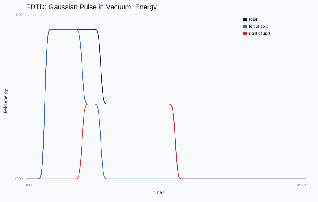
Stagger E on integer points and H on the half-points between them, and step them alternately. Both updates become centered second-order differences, and in vacuum at Courant number S \le 1 the scheme is non-dissipative — energy sloshes between E and H without decaying. It is to Maxwell what the mass-spring chain was to the scalar wave equation.

fig 3. A continuous source between two conductors: after many round trips the reflections superpose into a standing wave with stationary nodes — a 1D resonant cavity.

Reflection, refraction, resonance

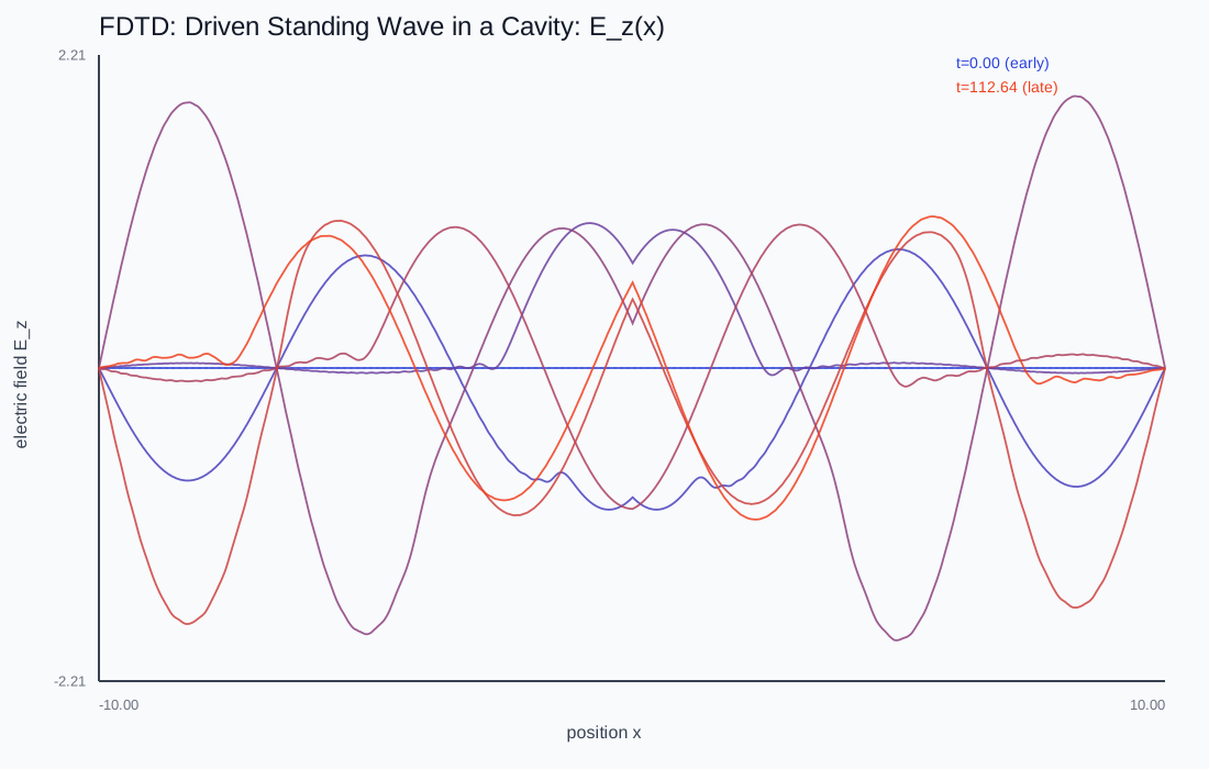
Absorbing (Mur) boundaries let a pulse leave the grid; a perfect conductor mirrors it with inversion. A dielectric interface splits a pulse with the exact Fresnel reflectance \big((n_1-n_2)/(n_1+n_2)\big)^2, and two conductors turn a continuous source into a standing-wave cavity — the electromagnetic echo of the fixed-fixed string.

fig 4. A pulse radiating in vacuum and leaving through absorbing ends: total field energy falls to zero as the light exits.

This chapter is drawn from the physics-lab study notes and renders. The longer write-ups and project essays live on the blog.